Mastering Day 21: What, Why & How
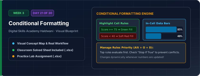
Dynamic visual formatting rules that automatically change cell background colors, fonts, or icons based on the values inside (e.g., green for profit, red for loss, yellow for pending).
Human brains process colors and visual patterns 60,000x faster than reading numbers. A manager can scan 500 rows in 3 seconds and spot overdue invoices or stock shortages instantly.
"Let colors speak! Conditional formatting is an automated highlighter pen that updates dynamically whenever numbers change."
What You Will Master Today
- Visual data alerting: automatically changing cell color based on numeric values
- Highlight Cells Rules: Greater Than, Less Than, Between, Equal To, Text that Contains
- Identifying and flagging duplicate entries in customer or employee rosters
- In-cell Data Bars for instant mini-bar chart visual volume comparison
- Color Scales (Green-Yellow-Red heatmap) for temperature or performance tracking
Step-by-Step Practical Walkthrough
Select the column of numbers you wish to format (e.g., Sales Revenue).
Go to Home tab > Conditional Formatting > Highlight Cells Rules > Greater Than.
Type your threshold value (e.g., 50000) and choose 'Green Fill with Dark Green Text'.
Click OK; any cell meeting your criteria instantly updates its color!
Haldwani Retail Store - Monthly Sales Performance with Visual KPI Flags
Study the completed reference worksheet below. Every column illustrates the standard formatting, formula structure, and alignment applied by professional office operators.
| Salesperson | Monthly Target (₹) | Achieved Sales (₹) | Performance % | Status Flag [Color Scale] |
|---|---|---|---|---|
| Rahul Joshi | 100000 | 124000 | 1.24 | Exceeded Target (Green) |
| Pooja Bisht | 100000 | 112000 | 1.12 | Exceeded Target (Green) |
| Deepak Rawat | 100000 | 94000 | 94.0% | Near Target (Yellow) |
| Sneha Arya | 100000 | 68000 | 68.0% | Below Target (Red) |
| Amit Negi | 100000 | 105000 | 1.05 | Target Met (Green) |
Student Attendance & Fee Arrears Audit
- Task 1: Highlight Column C (Attendance %): apply 'Highlight Cells Rules' > 'Less Than' 75 with Light Red Fill.
- Task 2: Highlight Column D (Fee Dues): apply 'Greater Than' 0 with Yellow Fill.
- Task 3: Apply in-cell Gradient Blue 'Data Bars' on Column C to visualize attendance volume.
- Task 4: Use 'Manage Rules' dialog to edit or remove any conflicting conditional rules.
Exercise Data Template Preview: Download the .xlsx file below and execute each task independently.
| Roll No | Student Name | Attendance % | Fee Dues (₹) | Exam Eligibility |
|---|---|---|---|---|
| 101 | Aman Rawat | 85 | ₹0.00 | Eligible |
| 102 | Bhumika Joshi | 68 | ₹4,500.00 | Short Attendance |
| 103 | Chandan Negi | 92 | ₹0.00 | Eligible |
| 104 | Deepika Arya | 72 | ₹8,500.00 | Fee Defaulter |
| 105 | Gaurav Bisht | 64 | ₹0.00 | Short Attendance |
Don't overload a spreadsheet with too many bright colors. Use soft pastel fills so your worksheets look executive and easy on the eyes!
Need 1-on-1 Guidance on Day 21?
Join our hands-on classroom lab sessions at Digital Skills Academy in Haldwani. Every student receives a dedicated PC workstation, live instructor reviews, and interview prep.